The Principles Behind Digital Image Sharpening
Sharpening as an Operation in the Frequency Domain
Sharpening
as an Operation in the Spatial Domain
Interpreting
the Inverse of the Blurring Matrix
Sharpening
as Executed by an Image Editing Program
Local
Contrast Enhancement and Sharpening by Unsharp Mask
Laplacian Edge Sharpening is Just More of the Same
Home
General Background
Optical imaging, recording, and reproduction systems are imperfect, and as a result, they
degrade and blur images. To the extent that degradation in image resolution is known and
is reproducible over the area of an image, often it can be reduced or reversed.
Generically, the inversion process is called sharpening, and purpose of the following
material is to explain how sharpening works.
Blurring and its inversion by sharpening can be analyzed in several ways. One basic
approach considers the spreading of a single sharp point of light. This form of analysis is
analogous to analyzing electronic circuits by their response to a sharp pulse input. The
second basic way to analyze blurring and sharpening considers images to consist of a sum
of signals that oscillate with varying position in the image. Low frequency components
describe properties that vary across large portions of an image and high frequency
components describe small details like the edges of objects.
Sharpening as an Operation in the Frequency Domain
A perfect lens faithfully images all details of an object.
That is, it perfectly transmits all
spatial frequencies without loss. A real lens may transmit low spatial
frequencies with an
efficiency near one, but it attenuates image information carried at the highest
frequencies.
For a nice discussion of the phenomenon, see
http://www.normankoren.com/Tutorials/MTF.html.
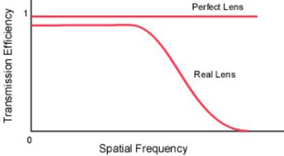
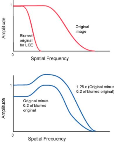
The loss of high frequency components produces blurring. If
the high frequency
components could be restored, then images would possess their normal contrast
for the
smallest objects, that is, they would be sharpened. In reality it is quite easy
to boost some
of the higher spatial frequencies and thereby improve the sharpness of an
image. The
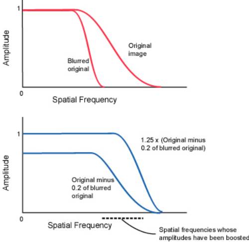
steps are the following:
1.
Blur a copy of the image. This destroys fine detail, that is,
it eliminates the
high spatial frequencies while it leaves gross features that are described by
low spatial frequencies largely unaltered.
2.
Subtract a fraction, say 0.2, of the blurred image from the
original. This
subtracts low frequency components from the original image while leaving the
high frequency components unaltered.
3.
Finally, boost the amplitude of all frequencies (contrast
enhancement). This
produces an end result in which the high frequencies have been boosted closer
to what a perfect lens would deliver, and the low frequencies remain as
before.
The procedure described above is the unsharp mask sharpening
method,
https://en.wikipedia.org/wiki/Unsharp_masking.
Clearly, the
radius used in the blurring step needs to be carefully chosen for optimum
results.
Sharpening
as an Operation in the Spatial Domain
To simplify the following discussion, images will be
considered as one dimensional. The
same principles and conclusions apply to two dimensional images. A one
dimensional
image can be represented as a set of pixel intensities along a line. Represent
these
intensities as a column vector where x1 provides the
intensity of the first pixel of the line,
x2 the intensity of the second, and so on.
![]()
![]()
A point object P that is positioned so that its image should fall on pixel 4 is represented as
 .
.
An imaging system somewhat blurs the point object P, and the
blurred image output B is
spread somewhat into adjacent line segments, perhaps as follows
 .
.
Represent the effect of the imperfect lens and sensor that
produced the above blurred
image as a matrix operator M acting on the point object vector P
to produce the blurred
output B,
![]() ,
,
or, writing out the matrices,
If other points along the original image line are similarly
blurred, for example, the next
point above the original point, then another column must be added to the left
of the center
of M. Hence, it is clear that the blurring matrix for a complete "image"
is the following.
So as to maintain total image intensity and to make
subsequent steps easier, the image
intensities that run off the edges of the matrix are piled up along the edges.
Of course, for
a real image thousands of pixels across, edge effects are negligible. The examples
shown
here have been chosen to be just large enough to display the general
properties.
In some cases, and this is one of them, the inverse of ![]() exists such that
exists such that ![]()
where I is the identity matrix with ones along the main diagonal and zeroes
everywhere
else. (![]() times any vector equals the vector.) The inverse of
times any vector equals the vector.) The inverse of ![]() in this case can be found
in this case can be found
with an ExcelTM spreadsheet and is
 .
.
In this case it is possible to reverse the blurring because
the blurred image, ![]() of a
of a
general object ![]() is
is ![]() and hence,
and hence, ![]() . That
. That
is, is the original image ![]() . Let us test this by applying our sharpening or
. Let us test this by applying our sharpening or
unblurring matrix ![]() to our blurred image. Multiplying our blurred point vector
to our blurred image. Multiplying our blurred point vector
by ![]() yields
yields
![]()
and except for round off errors, we recover the original image.
Areas of an image that possess uniform intensity ought not
to be changed by the
application of the sharpening matrix. This can be seen to be the case because
the sum of
the elements in each row is close to one. The sum of the elements in the
central row is
1.0000 when the more precise values in the spreadsheet are summed.
Interpreting the Inverse of the Blurring Matrix
The inverse of the blurring matrix that was determined in the previous section contains an
interesting prescription as to how to increase sharpness. Consider how the intensity of the
central pixel, pixel 4, in the blurred image contributes to the final unblurred image. For
pixel 1, examination of the unblurring matrix shows that the contribution of blurred pixel
4 to the final sharpened intensity of pixel 1 is 0.03 time the intensity of blurred pixel 4.
Similarly, the contribution of blurred pixel 4 to the sharpened intensity of pixel 2 is 0.14
times the intensity of blurred pixel 4. As expected, the strongest contribution of pixel 4 to
the sharpened image is to adjacent pixels 3 and 5, where it contributes -1.1 times the
intensity of pixel 4. This last contribution is nothing other than unsharp masking! That is,
the prescription for unsharp masking is to blur the image and subtract a portion from the
original. That is the same as what is accomplished by the matrix elements of value -1.1.
The unblurring or sharpening matrix ![]() contains the combined effects of subtracting a
contains the combined effects of subtracting a
portion of the blurred original and then multiplying the amplitude so as to
restore normal
contrast.
Photographers were not the first to invent the unsharp mask
procedure for sharpening
images. The human retina is hard wired to perform the unsharp masking
operation.
Psychologists call the phenomenon lateral inhibition,
https://en.wikipedia.org/wiki/Lateral_inhibition/
because exciting one
sensor in the eye slightly desensitizes nearby sensors. This is the same as
subtracting a
portion of the blurred image from the original. The halos which surround
objects
following aggressive sharpening of digital images also occur in human vision
where they
produce an optical illusion called Mach bands, https://en.wikipedia.org/wiki/Lateral_inhibition.
An interesting property of the unblurring matrix is the fact
that it contains instructions for
improving upon unsharp masking. That is, it also instructs us to ADD a portion
of the
intensity of pixel 4 to pixels 2 and 6 and a smaller portion to pixels 1 and 7.
One might
wonder whether the presence of both subtractive and additive terms in the
unblurring
matrix might be a special property dependent upon the precise shape of the
blurring curve
or blurring matrix. Experimenting with a wide collection of peak shapes for the
blurring
function shows that this is unlikely to be the case. Hence, this raises the
question, can the
unsharp mask sharpening algorithm usefully be improved upon by blurring a real
image
and subtracting a portion from the original, and then blurring with about twice
the
blurring radius and ADDING a smaller portion of this to the original?
Another question that the above analysis raises is whether
customizing a sharpening
algorithm to a particular picture significantly improves the results. In
principle, if one
knew that a particular feature in an image was the blurred image of a point
source, then
one could measure the intensities of nearby pixels and determine the elements
in the
blurring matrix. Inverting this should give the best possible method of
sharpening that
particular image.
Sharpening
as Executed by an Image Editing Program
The sharpening matrix can be deduced by applying it to a
suitable image because, as we
saw above,

will extract the values from M-1 giving the
contribution of the central pixel to surrounding
pixels. Since image editing programs do not record or use negative intensities
or
intensities above 1.0, a more useful "image" to process with a sharpening
procedure is
![]()
Picture Window ProTM. http://www.dl-c.com/
is an image editing program
designed for the serious photographer. Below are shown images prepared
with Picture Window Pro. The first is an enlarged view of an 11 pixel x 11 pixel "image"
in which the background has a luminosity of 0.2 and the central pixel has a luminosity of
0.6.

Sharpening not only lightens the central pixel, but it also
darkens surrounding pixels as
shown below. The exact values can be obtained with the program's readout tool.

Applying an unsharp mask also clearly lightens the central
pixel, but because more of the
surrounding pixels are darkened, the darkening effect is spread more thinly and
is less
conspicuous.

Local
Contrast Enhancement and Sharpening by Unsharp Mask
Images frequently can be brightened by increasing contrast.
Usually this cannot be done
globally because the process converts dark areas to pure black and light areas
to pure
white. Instead, techniques are used that enhance the contrast of light and dark
areas
differently. One method is to generate contrast masks so as to allow separate
manipulation of contrast in different parts of an image. While this method can
be
laborious, it can also yield beautiful results,
http://www.normankoren.com/PWP_contrast_masking.html.
There is, however, a rapid
global method for enhancing contrast that frequently gives good results.
Before describing how one uses an image editing program to
enhance contrast, it is
helpful to see how contrast can be increased without simply turning up contrast
on the
entire image. Consider an object in an image with features whose intensities
vary
between 9 and 10 units. The contrast in this area is then about one in ten. If
in this area of
the image we subtract five units of intensity and then multiply the intensities
by two,
points that previously had an intensity of nine, now have an intensity of
eight, and points
that previously had an intensity of ten still end with an intensity of ten. By
the subtract
and multiply operations, contrast has been increased from one in ten to two in
ten, that is,
it has been doubled. Similarly, if there are areas in the image with average
intensity of
100 and detail in this area has intensities between 90 and 100, then
subtracting 50 and
multiplying by two also doubles the contrast in these areas as well.
Blurring the original image discussed above with a radius on
the order of the major light
and dark objects in the image generates a new image with an intensity of about
10 in the
one area of the image and an intensity about 100 in the other area of the
image. That is,
the blurred image is what we need to subtract from the original. If half the
blurred image
is subtracted, and then the overall contrast is increased by a factor of two,
the local
contrast over most of the image is doubled.
The local contrast enhancement method just described above
boosts the amplitudes of the
higher frequency spatial components of an image by the same method that unsharp
mask
boosts the amplitudes of high frequency spatial components. In using the
unsharp mask
procedure to enhance local contrast, the radius for the blurring operation,
however, needs
to be chosen considerably larger than when the only objective is the sharpening
of edges.
The net result is that the amplitudes of some of the spatial frequencies are
increased well
above their natural values. When not done to excess, the process adds snap to
an image.
Typically a blur radius of a couple hundred pixels and an amplitude of about
20% is used.
Note that the process also boosts the amplitudes of the high frequency
components that
define edges. Thus, less edge sharpening is required after local contrast
enhancement,
LCE.
Laplacian
Edge Sharpening is Just More of the Same
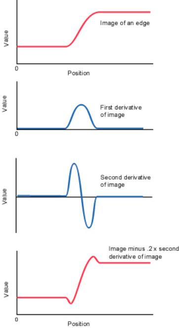
Sometimes sharpening is described in terms of the Laplacian
differential operator,
![]() , or in one dimension
, or in one dimension ![]() . At a slightly blurred edge, the
. At a slightly blurred edge, the
first and second derivatives of intensity would look roughly as shown, and when
a
portion of the second derivative is subtracted from the image, the end result
is a slight
halo and a sharpened edge.
The first derivative of intensity at the pixel i, xi, is the difference between the intensity of
xi+1 and xi, that is xi+1- xi divided by the
distance between i and i + 1 which we shall take
to be one. Similarly, the first derivative of the intensity at pixel i-1 is xi- xi‑1. The second
derivative of intensity at the origin is the difference of the first derivatives, and thus is
xi+1 - 2xi + xi-1.
If a portion of this second derivative is to be subtracted from the original
intensity, the operation is - xi+1 + 2xi
- xi-1 which is the by now familiar recipe for
subtracting a fraction of a pixel's intensity from the intensities of adjacent pixels.
August 2, 2005