The earliest ozone trend paper of which I am aware is Komhyr et al. [1971] in which they noted an apparent secular increase in ozone during the 1960s based on total column ozone measurements from a collection of ground-based Dobson spectrophotometers. The idea that ozone variability is dependent on meteorological conditions in the stratosphere goes back to a number of papers written in the decades before the Komhyr et al. paper. Discuss a number of papers on other effects on ozone.

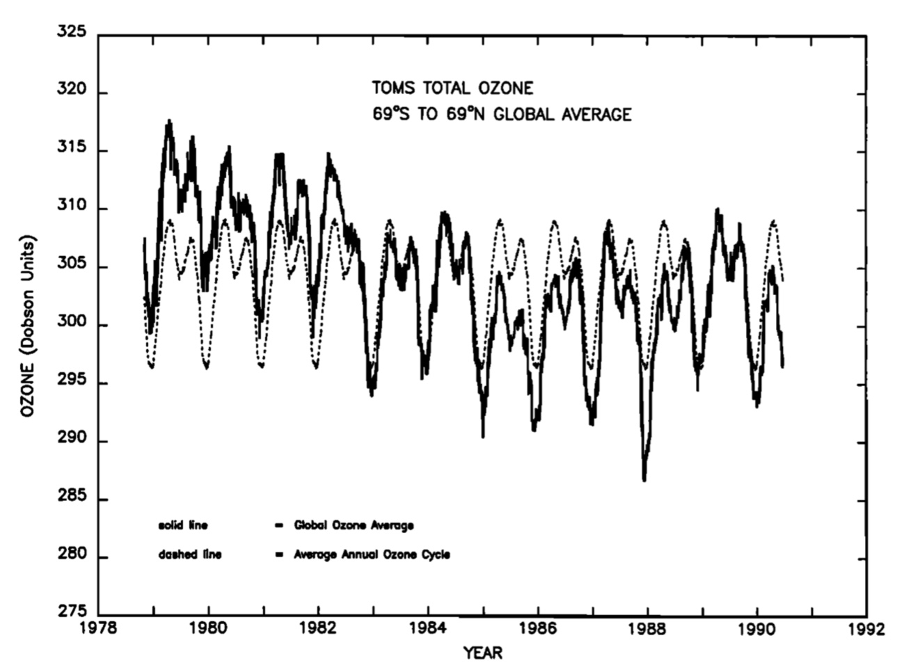
In 1991 we analyzed the recalibrated TOMS satellite data. The motivation for trend analysis and proxies was described by Herman et al. [1991]. Their results are described below with illustrations from that paper. The time series chosen to illustrate the long-term (not day-to-day or month-to-month) variation of ozone was the area-weighted integral of total column ozone between the latitudes of 69° South and 69° North. The limit at 69° avoids using highly-variable polar data where TOMS made no measurements during polar night. Averaging over the large swath of tropical and mid-latitude data averages out short-term variability that might obscure longer-term variations. In later works we have reduced the latitude range to 60°S-60°N to exclude more high latitude data.

Figure 3 from Herman et al. [1991] is shown below

	(Herman et al. Figure 3) Solid line shows the 69°S to 69°N area-weighted average of the monthly mean total ozone data from the TOMS instrument on the Nimbus 7 satellite. The dashed line shows average seasonal cycle deduced from the data.

We can then deseasonalize the time series by subtracting the mean seasonal cycle. The result below shows an apparent downward trend in the data

	(Herman et al. Figure 4) Solid line shows the result after removing the mean seasonal cycle. The dashed line shows a regression fit to a linear line illustrating the negative trend.

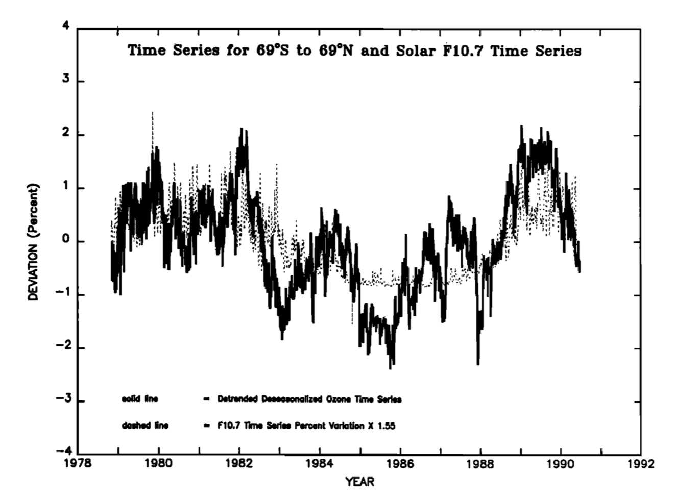
The residual after removing the linear trend is shown below

	(Herman et al. Figure 6) Solid line shows time series after removal of linear trend. Dashed line is the 10.7cm radio flux measured at Ottawa that we use as a proxy for the solar cycle.

This residual looks a lot like the 11-year solar cycle as represented by the 10.7cm radio flux measured at Ottawa shown by the dashed line. The next figure shows the difference between the solid and dashed lines, i.e. removing a solar cycle proxy from the data.

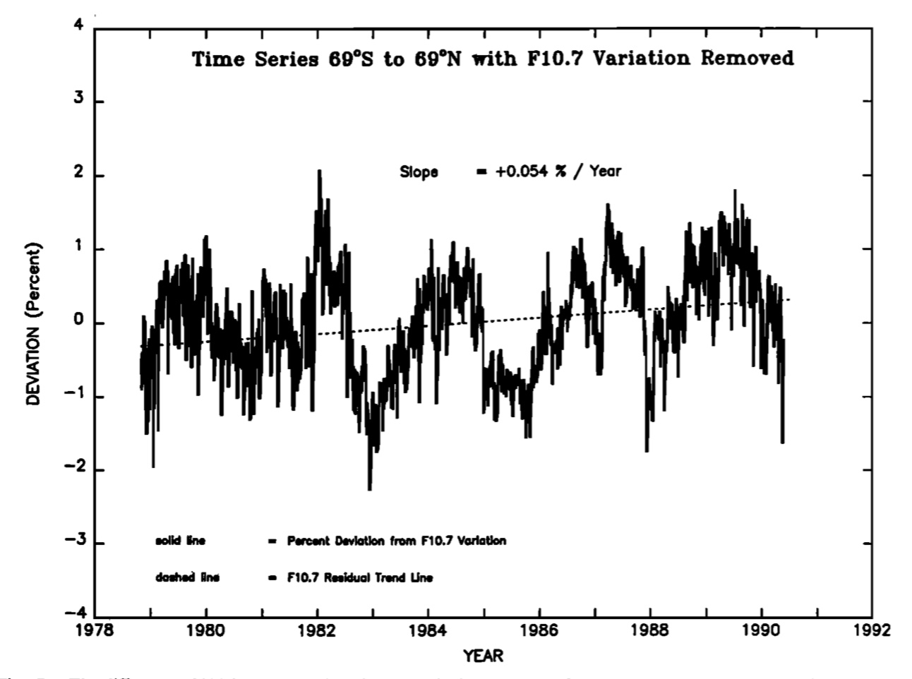
	(Herman et al. Figure 7) Solid line shows the residual after removal of the solar cycle. The dashed line shows a linear fit to the residual indicating that a small positive trend has been reintroduced into the data.

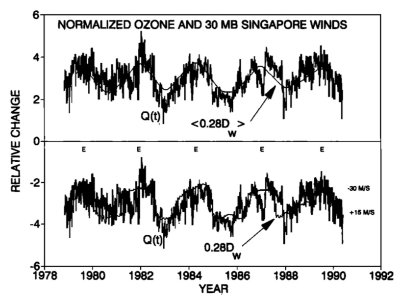
We see that a small positive trend has reappeared in the residual. This results from the trend in the solar cycle term. When we fit to trend and solar cycle simultaneously, this additional trend is automatically included in the deduced trend term. Here we have to take the two trend values and add them together to get the total trend in the data. After we remove this trend we have the result below, which looks very much like the quasi-biennial oscillation (QBO).

	(Herman et al. Figure 8) The solid lines in each panel are the residual after seasonal, trend, and solar cycle removal offset in the upper panel by 3 percent and in the lower panel by -3 percent. In each panel a representation of the QBO is superposed as a dashed line.

We then subtract off the QBO representation and note what is left. The next figure shows the ultimate residual in the lower part of the figure. It appears to be consistent with random, perhaps auto-correlated noise. The upper curves show the original deseasonalized data and the fit including all of the proxies described herein.

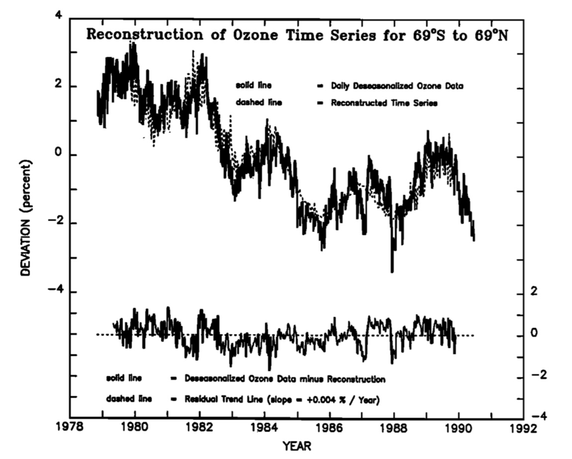
	(Herman et al. Figure 9) Upper solid curve shows the original time series with just the seasonal cycle removed. The upper dashed curve is the overall fit to that data using the proxies described. The lower curve is the residual difference between the data and the fit.

There has been a lot of improvement in our understanding of how to do time-series analysis of ozone data since the time of the Herman paper. The above presentation is meant to give the reader some background on the origin of the ideas behind the analyses. In the next section we will examine some of the proxies in more detail and give some history of our understanding of them.