Welcome to Ming Zhong's Homepage
Motivation: Main Research
As the observing technologies (sensors, cameras, camcorders, etc.) have matured over the years and the difficulties of data sharing have decreased, the amount of observation data has become immensely available (see this YouTube Video of swarm of starlings by National Geographic). My research is motivated by the need of making valid, useful and swift scientific discoveries from observation. For example, the story of how universal law of gravity was discovered traced back to Kepler's work on observation data of Mars' orbit.
To make a more precise statement of my research, the focus of my research is about designing and developing effective and efficient algorithms for making such discoveries. There are two major directions about my research:
- Infer dynamical structure from time-dependent obervations: Learning Dynamics
- Recover hidden variables from their noisy observations: Data Recovery
In order to make accurate, convergent, and effective algorithms, I use theories and techniques from machine learning, numerical ODE/PDE, scientific computing, approximation theory, inverse problems, probability and statistics. Oftentimes, due to the gigantic size of the data set, the algorithms have to be scalable and efficient, hence I employ various techniques which reduce computing time: multi-scale representation, iterative solver, dimension reduction, domain decomposition, parallel computing, GPU computing, (check out the Code section for details), etc. My research is interdisciplinary, it requries concrete knowledge of the observation technologies and underlying system, and it has applications in physics, biology, social science, and related engineering fields.
[ Back to top ]
Motivation: Data Recovery
How to recover unknown data from its observation, is one of the most interesting and challenging inverse problems. We consider two different cases in data recovery: recovery from observation when it is obtained via ill-conditioned observing operators together with observation noise, and recovery from observations obtained via observing operators when they depend on stochastic parameters.
In the case of recovery from observation obtained from ill-conditioned observing operators with noise, we mainly consider the family of regularization methods, especially the Tikhonov Regularization method and its variants, as one of the classical tools of solving and analyzing these data recovery problems (Compressed Sensing, Linear Regression and De-convolution). It is because the regularizing parameter can be considered as a resolution scale, which is the foundation for us to build our mulit-scale solver to on improve the traditional Tikhonov regularization approach. Another extra advantage of using such family of regularization methods is the flexibility of the method using the regularizing function, which adapts to the properties of the unknown quantities.
It is shown that the de-convolution problem on the discrete Helmholtz differential filter with noisy filtered data is an ill-posed linear inverse problem, where the ill-posedness increases along with the resolution of the Helmholtz solution. Realizing the information is still hidden in the residual, in [1], we combine the Lavrentiev regularization (a special case of Tikhonov regularization) to iterative refinement in order to solve the de-convolution of the discrete Hemlholtz differential filter from noisy data, which is commonly used in Large Eddy Simulation. An application of such approach combined with time-relaxation model for LES is studied in [2].
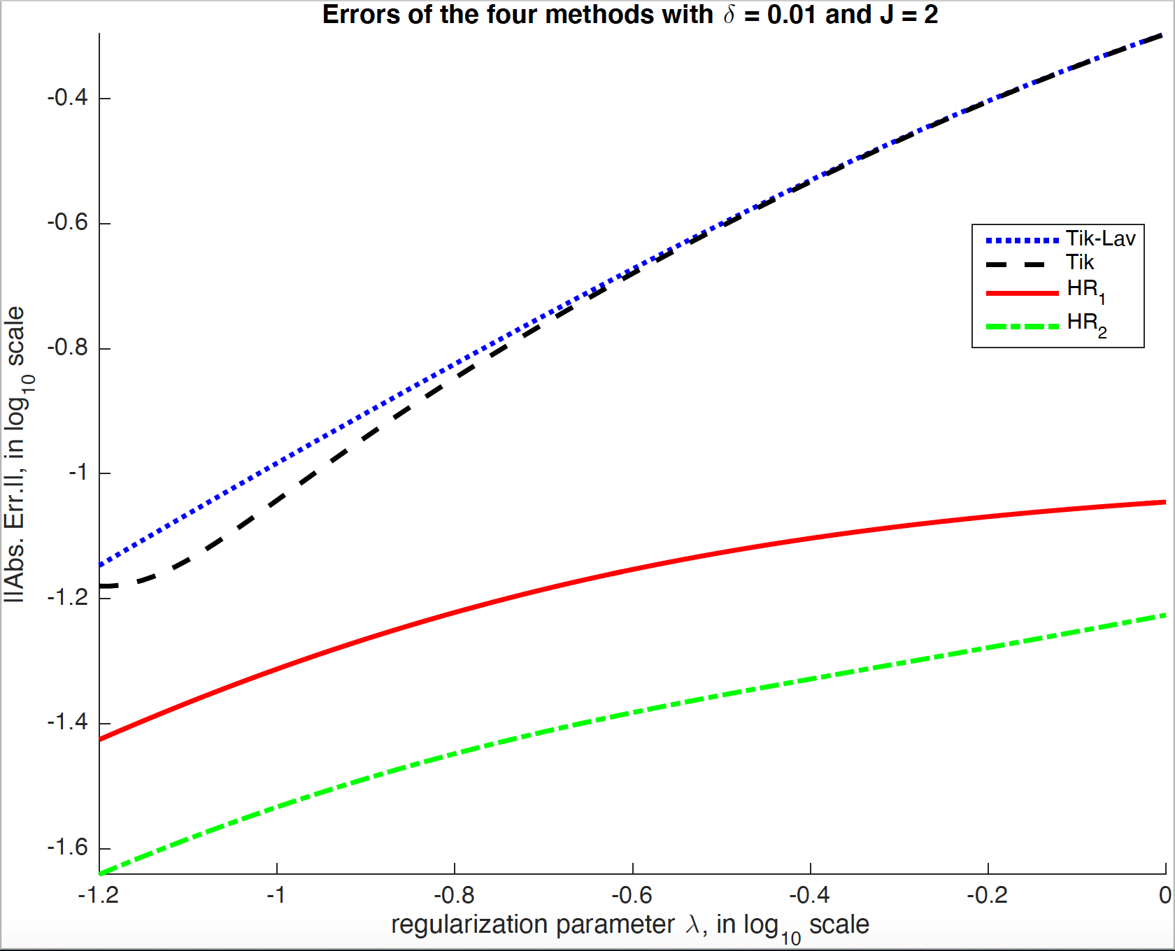
Recognizing the regularization parameter as a regularization scale, we extract de-coding information from the residual at different corresponding regualrization scales to arrive at a better solution to an ill-posed problems, which is the basic principle of the Hierarchical Reconstruction method. In [3], we combine the Tikhonov regularization with the Hierarchical Decomposition in order to tackle a series of prototypical data recovery problems: compressed sensing, linear regression, and de-convolution. In [4], we refined our analysis and sharpened the theoretical results. A refined error bond and deeper understanding of the l_1 error using the scaled residual is done on compressed sensing using the mono-scale LASSO method has been studied in [5].
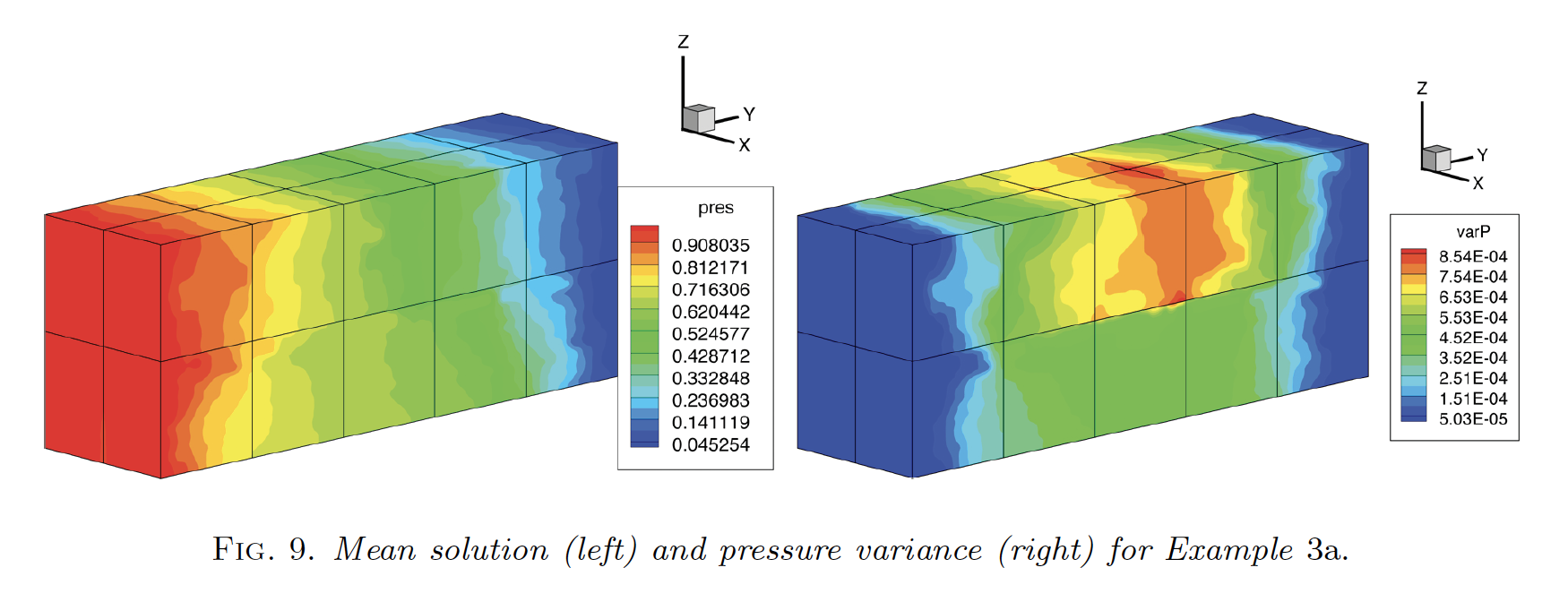
In the case of recovery from observation obtained via parametric observing operators with incomplete/stochastic information of the parameters, we are concerned about how uncertainty propagates through various science/eingeering based dynamical systems, where the dynamics are also controled by extra parameters. We consider the situation where the observation of these parameters are incomplete or random, making the corresponding dynamical systems stochastic. In order to gain useful insight about the solutions of the stochastic dynamical systems, we consider the first two moments (mean and variance) of the stochastic solutions, which results in evaluating integrals over high-dimension spaces. To avoid the curse of dimensionality from using a simple Tensor Grid of abscissas and weights, we consider two different kinds of dimension reduction techniques used in evaluating integrals over a high dimension space: Monte Carlo and Sparse Grid. Details can be found about applying Monte Carlo/Sparse Grid to solve Darcy's equation with stochastic permeability can be found in [6].
List of publications in Data Recovery:
- N. Mays, M. Zhong. Iterative Refinement of a Modified Lavrentiev Regularization Method for De-convolution of the Discrete Helmholtz type Differential Filter, ArXiv e-prints, January 2018.
- M. Zhong. Time Relaxation with Iterative Modified Lavrentiev Regularization, ArXiv e-prints, September 2018.
- M. Zhong. Hierarchical Reconstruction Method for Solving Ill-posed Linear Inverse Problems, Ph.D. Thesis, May 2016.
- E. Tadmor, M. Zhong. The Multi-scale Hierarchical Reconstruction of Ill-posed Inverse Problems, In Preparation.
- E. Tadmor, M. Zhong. Sparse Recovery of Noisy Data Using the LASSO Method, submitted (arXiv page).
- B. Ganis, I. Yotov, M. Zhong. A Stochastic Mortar Mixed Finite Element Method for Flow in Porous Media with Multiple Rock Types, SIAM J. Sci. Comp., 33 (3), 1439 - 1474, June 2011.
[ Back to top ]
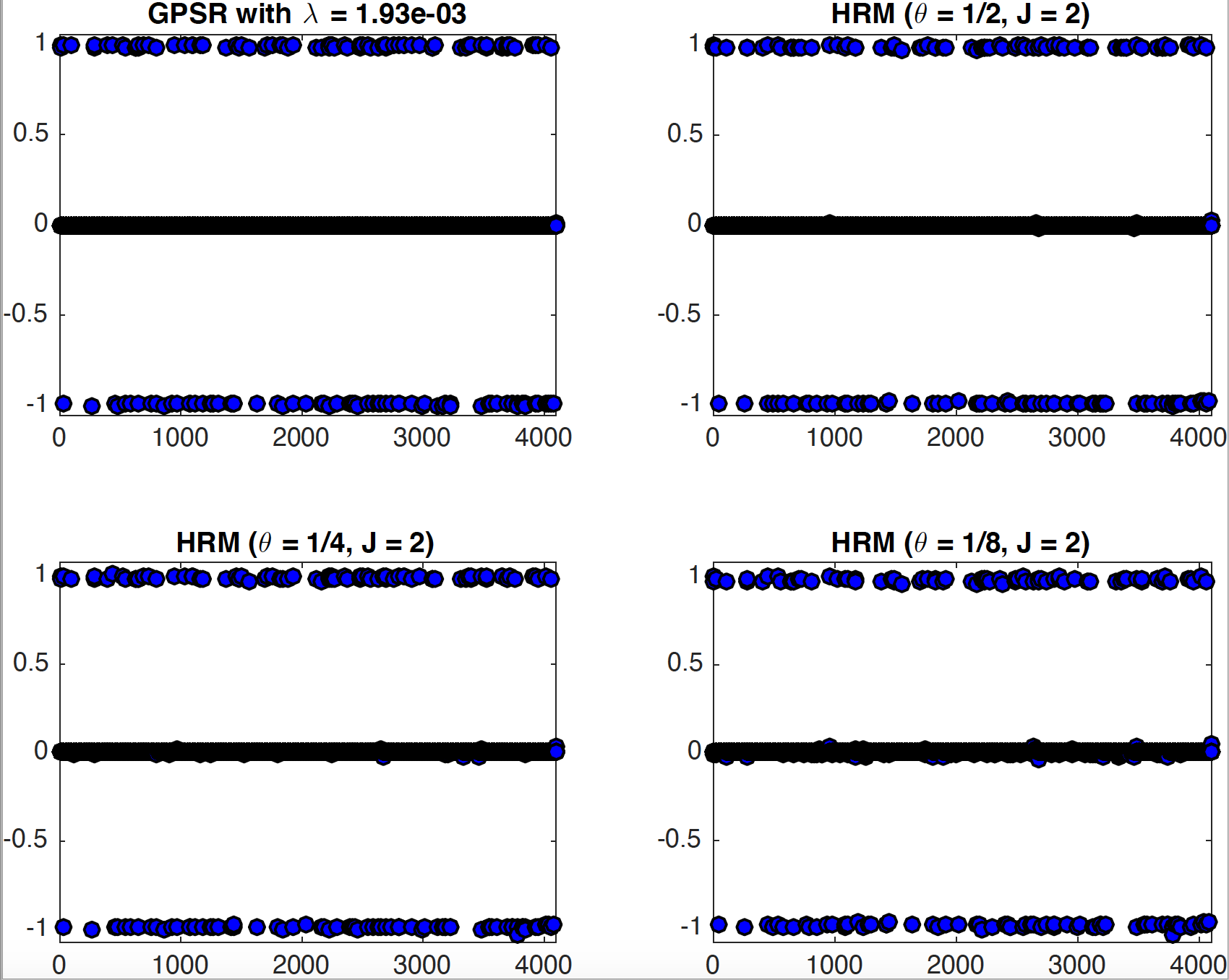
Examples -- Compressed Sensing
Compressed Sensing concerns about recovering unknown signals/images using undersampling techniques. The Nyquist-Shannon sampling theorem gave a lower bound on the sampling rate on how to recover unknown signals/images perfectly. However when combined with ''a priori'' knowledge of the sparisty of the unknown signals/images, one can use fewer (fewer than the Nyquist rate) number of samples to recover the unknown. Early 2000, E. Candes, J. Romberg, and T. Tao (separately D. Donoho) showed that given the sparsity level of the unknown, the unknown quantity can be re-constructued with the number of samples being around the level of sparsity, when the sampling/observing/measuring operators (or matrices) satisfy one of the following three properties: Restricted Isometry Property (known as RIP in E. Candes, J. Romberg, and T. Tao's paper, ''Robust Uncertainty Principles: Exact Signal Reconstruction from Highly Incomplete Frequency Information''), L-1 coherence (D. Donoho and X. Huo's paper, ''Uncertainty Principles and Ideal Atomic Decompositions''), and Null Space Property (known as NSP in A. Cohen, W. Dahmen and R. DeVore's paper, ''Compressed Sensing and the Best k-term Approximation).
Another important discovery of the Compressed Sensing theories is that the convex L-1 norm can be used to replace the non-convex L-0 norm. L-1 constrained optimizations have seen a great number of applications: matching pursuit in 1993, LASSO in 1996, and basis pursuit in 1998. We are particularly interested in Tikhonov regularization method with L-1 norm as the regualrizing function.
Result from using Hierarchical Reconstruction method.
[ Back to top ]
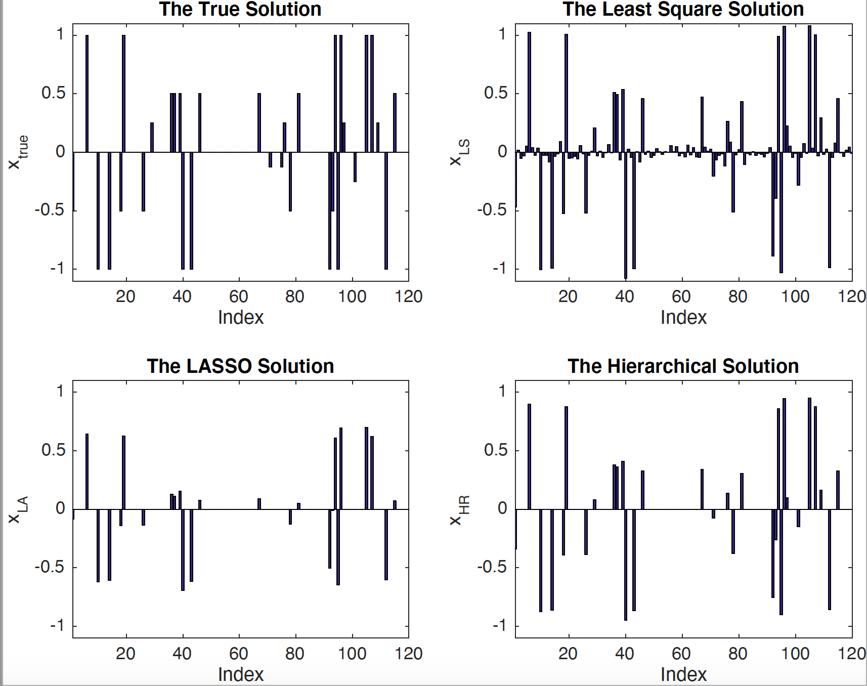
Examples -- Linear Regressoin with LASSO
Linear Regression is a linear approach to infer the relationship between the response variables and the explanatory variables. The relationship is called a model. In the case of linear regression, one has to learn the linear models to explain the dependence and independence variables. However, when the dimension of the linear model grows too large, one has to find an easier way to explain the model. LASSO combines linear regression with sparse recovery, hence a sparse linear model is learned by the LASSO approach, which makes the sparse linear model much easier to explain than an usual linear model from any L-2 based approach.
Result from using Hierarchical Reconstruction method.
[ Back to top ]
Examples -- De-convoluton of Discrete Helmholtz Differential Filter
De-convolution is the reverse procedure to clean the effect of convolution on signals/images. We are interested in the convolution by a particular filter, the Helmholtz differential filter, which is a popular filter used in Large Eddy Simulation, due to the filter's explicit de-convolution procedure. However, in the actual applications, a discrete approximation of the filter is used, and the filtered quantities are corrupted by various kinds of noise. How to obtain the unfiltered solution in the discrete setting becomes a challenge, and the approximation resolution of the filter, the filter length, and the regularity of the filtered quantities all play a role in obtaining a reasonable recovery.
Result from using Hierarchical Reconstruction method.
[ Back to top ]
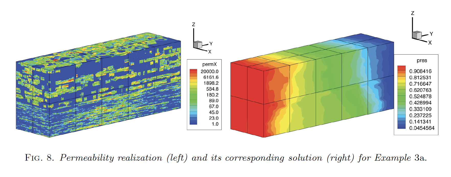
Example: Darcy's Law with Random Permeability
Next we consider the linear equation, Ax = b, in the context of solving a linear ellitic PDE with boundary conditions. However, we also consider that A depends on some parameter k, but we have incomplete information of k, hence making k stochastic. Then in order to solve for each x for one realization of k, we obtain statistics of x based on the information on k. However, the integrals to obtain the statistics of x are high-dimensional, hence certain dimension reduction techniques have to be used.
We consider an applicaiton of our approach: by solving the Darcy's Law with a stochastic permeability for modeling underground water flow over a large physical domain. The random permeability is approximated using a finite KL-expansion. In order to reduce the computing time, domain decomposition is used. With implementation in MPI and FORTRAN 77, we were able to test our algorithm on the SPE10 (a benchmark problem for reservoir simulation).